Detecting Independence
In Neural Conditional Probability for Uncertainty Quantification (Kostic et al., 2024), the authors claim that the (deflated) conditional expectation operator can be used to detect the independence of two random variables X and Y by verifying whether it is zero. Here, we show this equivaliance in practice.
Dataset
We consider the data model
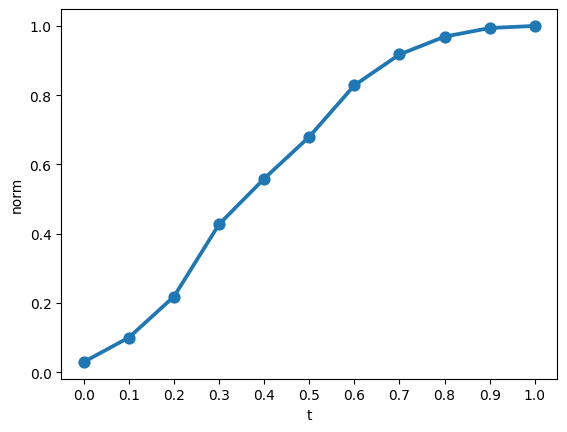
where \(X\) and \(X'\) are independent standard Gaussians in \(\mathbb{R}\), and \(t \in [0,1]\) is an interpolating factor. This model allows us to explore both extreme cases (\(t = 0\) for independence and \(t = 1\) where \(Y = X\)) and the continuum in between, to assess the robustness of NCP in detecting independence.
import torch
from torch.utils.data import DataLoader, TensorDataset, random_split


def make_dataset(n_samples: int = 200, t: float = 0.0):
    """Draw sample from data model Y = tX + (1-t)X_, where X and X_ are independent gaussians.

    If t = 0, then X and Y are independent. Otherwise, if t->1, X and Y become ever more dependent.

    Args:
        n_samples (int, optional): Number of samples. Defaults to 200.
        t (float, optional): Interpolation factor. Defaults to 0.0.
    """
    X = torch.normal(mean=0, std=1, size=(n_samples, 1))
    X_ = torch.normal(mean=0, std=1, size=(n_samples, 1))
    Y = t * X + (1 - t) * X_

    ds = TensorDataset(X, Y)

    # Split data into train and val sets
    train_ds, val_ds = random_split(ds, lengths=[0.85, 0.15])

    return train_ds, val_ds
Learning the conditional expectation operator
Now, we go through the process of learning the conditional expectation operator \(\mathbb{E}_{Y \mid X}: L^2_Y \mapsto L^2_X\)
where \(g \in L^2_Y\). We begin by noting that, if \(\{u_i\}_{i=1}^\infty\) and \(\{v_j\}_{j=1}^\infty\) were orthonormal bases of \(L^2_X\) and \(L^2_Y\) (Orthonormal basis wikipedia), then we could see the conditional expectation operator as an (infinite) matrix \(\mathbf{E}\), where
Hence, to learn the operator, we “only” need to learn the most important parts of \(\mathbf{E}\). The standard way to deal with such problems is to restrict oneself to finite subspaces of \(L^2_X\) and \(L^2_Y\) and then learn the (finite) matrix there. This corresponds to finding orthonormal functions \(\{u_i\}_{i=1}^d\) and \(\{v_j\}_{j=1}^d\) s.t.
is minimized, where \(d \in \mathbb{N}\) is the dimension and \(\mathbb{E}_{Y \mid X}^d\) is the truncated operator that acts on \(span\{v_j\}_{j=1}^d\) and \(span\{u_i\}_{i=1}^d\). The theoretical solution of this problem is given by the truncated (rank d) Singular Value Decomposition (Low-rank matrix approximation wikipedia), which also has the nice benefit of ordering the bases by their importance a la PCA, meaning that \(u_1\) is more important than \(u_2\), and so on and so forth.
A representation learning problem
A key insight of Kostic et al. (2024) is that this problem corresponds to a representation learning problem, where the goal is to find latent variables \(u,v \in \mathbb{R}^d\) that are
(Whitened, wikipedia): \(\mathbb{E}[u_i(X)u_j(X)] = \mathbb{E}[v_i(Y)v_j(Y)] = \delta_{ij}\); and
Minimize the contrastive loss
where \(S\) is the matrix of the conditional expectation operator on these subspaces/features, which can be learned end-to-end with backpropagation or estimated with running means.
Representation learning in Torch
from torch.nn import Module
import torch
import math
from torch import Tensor


class _Matrix(Module):
    """Module representing the matrix form of the truncated conditional expectation operator."""

    def __init__(
        self,
        dim_u: int,
        dim_v: int,
    ) -> None:
        super().__init__()
        self.weights = torch.nn.Parameter(
            torch.normal(mean=0.0, std=2.0 / math.sqrt(dim_u * dim_v), size=(dim_u, dim_v))
        )

    def forward(self, v: Tensor) -> Tensor:
        """Forward pass of the truncated conditional expectation operator's matrix (v -> Sv)."""
        # TODO: Unify Pietro, Giacomo and Dani's ideas on how to normalize\symmetrize the operator.
        out = v @ self.weights.T
        return out


class NCP(Module):
    """Neural Conditional Probability in PyTorch.

    Args:
        embedding_x (Module): Neural embedding of x.
        embedding_dim_x (int): Latent dimension of x.
        embedding_y (Module): Neural embedding of y.
        embedding_dim_y (int): Latent dimension of y.
    """

    def __init__(
        self,
        embedding_x: Module,
        embedding_y: Module,
        embedding_dim_x: int,
        embedding_dim_y: int,
    ) -> None:
        super().__init__()
        self.U = embedding_x
        self.V = embedding_y

        self.dim_u = embedding_dim_x
        self.dim_v = embedding_dim_y

        self.S = _Matrix(self.dim_u, self.dim_v)

    def forward(self, x: Tensor, y: Tensor) -> Tensor:
        """Forward pass of NCP."""
        u = self.U(x)
        v = self.V(y)
        Sv = self.S(v)

        return u, Sv
Training NCP
We now how to train the NCP module above with the contrastive loss from linear_operator_learning.nn with orthonormality regularization and standard deep learning techniques.
from torch.optim import Optimizer

def train(
    ncp: NCP,
    train_dataloader: DataLoader,
    device: str,
    loss_fn: callable,
    optimizer: Optimizer,
) -> Tensor:
    """Training logic of NCP."""
    ncp.train()
    for batch, (x, y) in enumerate(train_dataloader):
        x, y = x.to(device), y.to(device)

        u, Sv = ncp(x, y)
        loss = loss_fn(u, Sv)
        loss.backward()
        optimizer.step()
        optimizer.zero_grad()
import torch
import linear_operator_learning as lol


SEED = 1
REPEATS = 1
BATCH_SIZE = 256
N_SAMPLES = 5000
MLP_PARAMS = dict(
    output_shape=2,
    n_hidden=2,
    layer_size=32,
    activation=torch.nn.ELU,
    bias=False,
    iterative_whitening=False,
)
EPOCHS = 100
WHITENING_N_SAMPLES = 2000

torch.manual_seed(SEED)

# device = torch.accelerator.current_accelerator().type if torch.accelerator.is_available() else "cpu"
device = "cpu"
print(f"Using {device} device")

results = dict()
for t in torch.linspace(start=0, end=1, steps=11):
    for r in range(REPEATS):
        run_id = (round(t.item(), 2), r)
        print(f"run_id = {run_id}")

        # Load data_________________________________________________________________________________
        train_ds, val_ds = make_dataset(n_samples=N_SAMPLES, t=t.item())

        train_dl = DataLoader(train_ds, batch_size=BATCH_SIZE, shuffle=False)
        val_dl = DataLoader(val_ds, batch_size=BATCH_SIZE, shuffle=False)

        # Build NCP_________________________________________________________________________________
        ncp = NCP(
            embedding_x=lol.nn.MLP(input_shape=1, **MLP_PARAMS),
            embedding_dim_x=MLP_PARAMS["output_shape"],
            embedding_y=lol.nn.MLP(input_shape=1, **MLP_PARAMS),
            embedding_dim_y=MLP_PARAMS["output_shape"],
        ).to(device)

        # Train NCP_________________________________________________________________________________
        loss_fn = lol.nn.L2ContrastiveLoss()
        optimizer = torch.optim.Adam(ncp.parameters(), lr=5e-4)

        for epoch in range(EPOCHS):
            train(ncp, train_dl, device, loss_fn, optimizer)

        # Extract norm______________________________________________________________________________
        x = torch.normal(mean=0, std=1, size=(WHITENING_N_SAMPLES, 1)).to(device)
        x_ = torch.normal(mean=0, std=1, size=(WHITENING_N_SAMPLES, 1)).to(device)
        y = t * x + (1 - t) * x_
        u, Sv = ncp(x, y)

        _, _, svals, _, _ = lol.nn.stats.whitening(u, Sv)
        results[run_id] = svals.max().item()
Using cpu device
run_id = (0.0, 0)
run_id = (0.1, 0)
run_id = (0.2, 0)
run_id = (0.3, 0)
run_id = (0.4, 0)
run_id = (0.5, 0)
run_id = (0.6, 0)
run_id = (0.7, 0)
run_id = (0.8, 0)
run_id = (0.9, 0)
run_id = (1.0, 0)
Plots
import pandas as pd
import seaborn as sns

results_df = pd.DataFrame(
    data=[(t, r, norm) for ((t, r), norm) in results.items()],
    columns=["t", "r", "norm"],
)
sns.pointplot(results_df, x="t", y="norm");